This post originally appeared on the Coalmarch blog in 2015 (Coalmarch is a former employer of mine). They were going to remove it, but asked if I wanted to move the post to my site. So I did! The following is the original blog post, with one new section at the end if you want to get extra fancy.
———————————————————————————————
We use the “IMPORT RANGE” function in Google Sheets frequently. It’s crucial when trying to work with the behemoth of admin documents we have. Luckily, it’s a pretty straightforward function. All it does is pull in a cell from another sheet into the sheet we’re working in. But, there’s one problem with it: if you’re working with a big document and you want to fill the function down or across, it doesn’t work. Luckily, I found a solution!
First, in case you don’t use it, let me show you how it works.
The IMPORT RANGE Function
Google will tell you that the function looks like this:
=IMPORTRANGE(spreadsheet_key, range_string)
Here’s what that means:
spreadsheet_key: Every Google Sheet has a URL that looks something like this (“https://docs.google.com/spreadsheets/d/1vXc1-xuRjdUmakIO5jvuOe4qcbcASPF_…“). The spreadsheet key is that string of gibberish after the /d/. So, in the case above, 1vXc1-xuRjdUmakIO5jvuOe4qcbcASPF_axvWDVsY9h26p0.
range_string: This is just the cell from the target sheet that we’re looking to import into our working sheet. We’ll need to include the sheet name and the cell name. So, if we want to pull what’s in cell A1 from our target sheet called “New Document”, we’d just use the standard notation of New Document!A1.
Putting it together, this is what our function would look like (notice that both parts of the function have to be surrounded with double quotes):
=IMPORTRANGE(“1vXc1-xuRjdUmakIO5jvuOe4qcbcASPF_axvWDVsY9h26p0”, “New Document!A1”)
That’s it! So here’s an example. I have three documents I’m working on. Test Doc 1, 2, and 3. Doc 2 has client contact name information in it, Doc 3 has client location information in it, and I want Doc 1 to be a hub that has both contact name and location information in it.


We could manually copy and paste the info from 2 and 3, but if we change those frequently, we may want to have it dynamically pull that information. So, we use IMPORT RANGE.
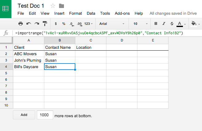
So let’s grab the “Contact Name” info from Test Doc 2. To do so, I went to Test Doc 2 and grabbed the spreadsheet key from the URL, the sheet name, and note that I want to pull the first contact name, which is at cell B2.

So my formula in cell B2 of Test Doc 1 looks like this:
=IMPORTRANGE(“1vXc1-xuRjdUmakIO5jvuOe4qcbcASPF_axvWDVsY9h26p0”, “Contact Info!B2”)

Then, hit enter. The first time a spreadsheet tries to communicate with another spreadsheet, we’ll have to authorize access between them:
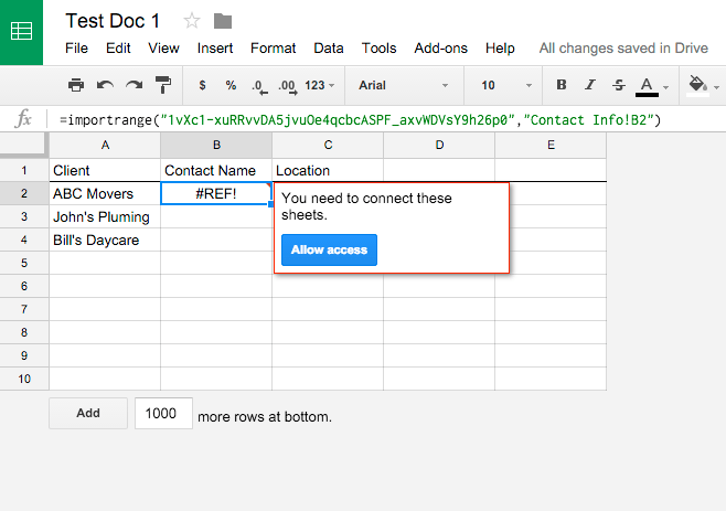
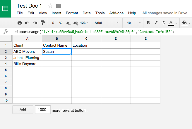
Once we do that, we should see the data from our other sheet!
So here’s the tricky part. Normally with a function, we’d be able to “fill” it down and it would change the function to match the new area. I’ll show you an example.
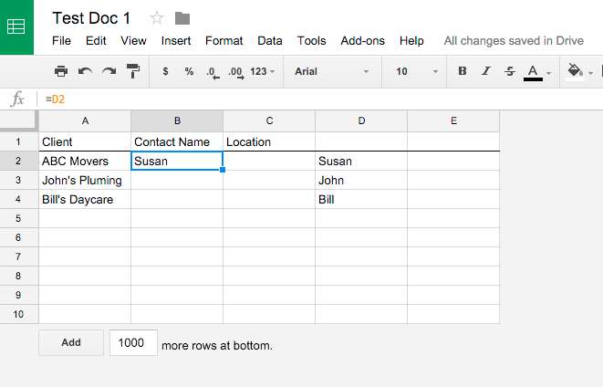
Let’s say instead of referencing a different sheet, the client names were in the same sheet but just in a different column and we were just referencing them there. In that case, the formula would just refer to the other column, or in this case, it would be “=D2”:
If we fill that down, it will fill the rows correctly:
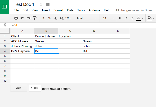
Notice how the new formula changed from “=D2” in row 2 to “=D4” in row 4. But if we try to do that with the IMPORT RANGE function, nothing changes. It imports the same cell every time:
The reason is in the name of that part of the function: range string. A string is text–it’s not a row or column or number like a function normally has. A spreadsheet can tell what you’re doing when you try to fill a formula down that is referencing a cell–you probably want the formula to reference the cells below the original. If you’re filling it to the right, you probably want it to reference the cells to the right of the original.
If it’s a string, it can’t tell that you’re referencing a cell, it just sees the letters and numbers that make up “Contact Info!B2”.
So. How do we dynamically reference that cell so that it fills correctly?
The ADDRESS, COLUMN, and ROW Functions
The answer is a function called ADDRESS. It’s a pretty meta function. Google says it “returns a cell reference as a string” when you input the row and column. So say you tell it row 1, column 1, it will return “A1”, but it will return it as a string and not the actual cell. Sound familiar? That’s exactly what we need for the “range string” part of the IMPORT RANGE function to work.
Here are the full details of the address function. It looks like this:
=ADDRESS(row, column, [absolute_relative_mode], [use_a1_notation], [sheet])
That means:
row: Simply, the row number you’re referencing.
column: The column you’re referencing. Keep in mind this is a number not a letter, so A would be 1, B would be 2, etc.
[absolute_relative_mode]: This is optional. You can tell the function whether you want it to use absolute or relative references. I leave this out.
[use_a1_notation]: Also optional. You can use A1 or standard (R1C1) notation. I leave this out as well.
[sheet]: Also optional, but this one is useful. You can tell it the name of the sheet you’re looking for in case there are multiple sheets in the doc you’re pointing to.
So if we want the B2 cell in Test Doc 1 to grab the B2 cell in Test Doc 2, we just need the range string in our IMPORT RANGE function to reference the current row and column. Luckily, there’s a simple way to do that using the ROW and COLUMN functions. If you use the formulas of just “=ROW()” and “=COLUMN()” with nothing in the parenthesis, you’ll get the row and column of the cell you’re currently in.
You can see this below. I added the ROW functions to cells D2, D3, D4, and D5 and it gave me the row numbers. I added the COLUMN functions to C6, D6, and E6 and it gave me the column numbers.

This means we can use these formulas within the ADDRESS function. The final formula would look like this:
=ADDRESS(ROW(),COLUMN(),,,”Contact Info”))
Which just means “give me the address of the cell in the “Contact Info” sheet of the same row and column of where I currently am.” Note that commas separate each part of the function, so because we’re skipping the first two optional parts, you have to put three commas in between the column and the sheet name.
So, to pull it all together, we can use this in our IMPORT RANGE:
=IMPORTRANGE(“1vXc1-xuRRvvDA5jvuOe4qcbcASPF_axvWDVsY9h26p0″,ADDRESS(ROW(),COLUMN(),,,”Contact Info”))
We can now fill this down and it will work perfectly. The row() and column() functions change when we fill it down and it returns the range string the IMPORT RANGE function needs.

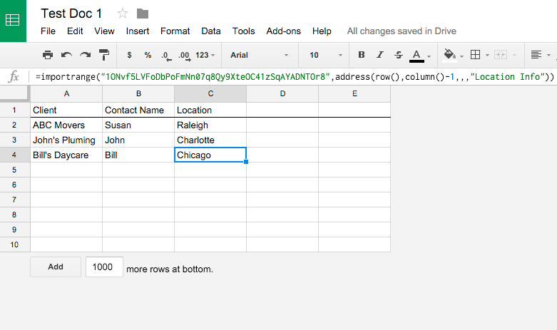
One last trick. The third column isn’t going to work like this because the column (C) doesn’t match up to where you want to grab the info from in Test Doc 3 (B). So, a simple edit of the IMPORT RANGE function is all it takes (the change is bolded):
=IMPORTRANGE(“1ONvf5LVFoDbPoFmNn07q8Qy9XteOC41zSqAYADNTOr8”,ADDRESS(ROW(),COLUMN()-1,,,”Location Info”))
We’re referencing a different spreadsheet, so I updated the spreadsheet key and sheet name. But, the tricky part is that “column()” is now “column()-1”. The orginial “column()” would have returned a 3 (meaning C) but we want a 2 (meaning B), so a simple minus one gets us there.
The final doc:
That’s it! Our doc will automatically update and we’ll be able to fill the formulas down if we add new rows in the future.
If I’m missing anything or if you’ve tried this and it doesn’t work, email me and I’ll help you out!
Cheers!
</end of original post>
———————————————————————————————
New Stuff!
As I was porting this over, I realized two things:
1) Linking to the example docs may help some people, so here they are:
2) You can make this example a little faster if you had an especially large spreadsheet with many columns. So, in the “Test Doc 3”, the original setup is in the “Simpler” tab, but I added two “Fancier” tabs. The “Fancier (Reference)” tab is a table for VLOOKUPS and the “Fancier (Final)” tab is the original table using those VLOOKUPs.
The Fancier version just makes it so that you don’t have to write different formulas for each column–as long as you include the lookup data in the “Reference” tab, you can have as many columns as you want and you only need one formula.
Cheers!
Thanks for info – I use importrange a lot, and assumed that it dynamically linked the files (sheets). But, I was just re-importing a table into a source sheet which is imported into some other sheets via lookups, etc. The data in the destination sheets didn’t change to match the new export!? Not at first anyway. Then, perhaps 15 mins later, it did. I wonder if you are familiar with this sort of glacial latency in such linked google sheets?
Hey Hudson. Glad to help. Yes, I would expect a few minutes delay when updating a web of documents like that. 15 seems a bit high, but that would just depend on how slow Google Apps is that day, I suppose?
Hi Lee,
I’ve successfully done the “importrange” using this method for the first spreadsheet. But the 2nd, 3rd and 4th is not coming through. Could you have a quick look at my formulas?
Hey Col. Glad to. Jot them down here and I’ll take a look.
Lee.
This sheet is where I am importing date from 4 others sheets:
The formula below is working fine to import data from cells D1 to H23.
=IMPORTRANGE(“https://docs.google.com/spreadsheets/d/1bl4LgXs06RcOX6g0hwAS19fJNUIaGFWo8pEhFVOM3Ns/edit#gid=0″;ADDRESS(row();column();;;”Sheet1”))
But it is not working for cells d24 to h46 for data importing from the 2nd sheet for this formula =IMPORTRANGE(“https://docs.google.com/spreadsheets/d/1JOnJkVKrR3_5gYbw9TT_bbD0WxQoU986SusuYQkc1uI/edit#gid=0″;ADDRESS(row();column();;;”Sheet1”))
Same for 3rd sheet using =IMPORTRANGE(“https://docs.google.com/spreadsheets/d/10OpIhXUnvZFI5_ySktOn-Wr_6aIVP2w2rCkViIOWVAs/edit#gid=0″;ADDRESS(row();column();;;”Sheet1”))
and 4th sheet for
=IMPORTRANGE(“https://docs.google.com/spreadsheets/d/1ZR8bkZIhxj_wQGyjBCN72W0UsAS771FzhH192l5n-JQ/edit#gid=0″;ADDRESS(row();column();;;”Sheet1”))
Hey Col I took a quick look–everything seemed to be fine on the two docs I had access to. I can’t imagine why that wouldn’t work! Can you give me access to the two other docs?
Hey Col–Is there a 5th document too? Actually, why don’t you email me (lee@leelkennedy.com) and I’ll help you out that way–that will be much easier.
Whoever you are, wherever you live, I will forever owe you “bigly” Lee Kennedy.
You just made my day!
Ha! Glad to help, Omar.
Hey Lee,
This is amazing! Thanks for sharing and keep it alive 🙂 I have an IMPORTRANGE running and importing data from 4 sheets sitting in the same google sheet in a MasterSheet (Data stacked one data set on top of another ). The thing is it leaves blanks in between … so I wonder how to make it stop importing from sheet1 once no data is populated in Sheet1!, so it sticks directly DATA from sheet2! not leaving blanks in between? Is it possible with IMPORT RANGE or I should use a Query please?
Thanks Lee
Kamar
Hey Kamar. Glad it helped. I’m not sure you’d be able to limit the IMPORTRANGE like that unless you somehow dynamically were able to pull in the range of non-blank cells. It’s likely possible, but I’d have to see it. A QUERY function might be a better idea as long as it doesn’t slow everything down too much.
I’ve been using importrange in a google doc for a few weeks and it is working as expected, although with one issue for which I can’t find an answer.
Let’s use your Test Doc 1 as an example, and all the imported Client, Contact and Location info is being imported just fine. Let’s also say that the spreadsheet_key references a doc which you don’t maintain, so you are unable to create a new column there.
Now, in your Test Doc 1, you create a new column labeled “Sent Birthday Gift” and manually enter “yes” or “no” in each respective cell.
Remember, this column is not part of the original spreadsheet_key you are referencing, so it isn’t data you can import and has to be manually created.
Here’s my issue…each time a new row (Client, Contact Name and Location) is imported from the original doc, it pushes the previously imported data down one row. However, the manually added data (yes/no) in the Sent Birthday Gift column is now out of position.
How can the manual data preserve its position in relation to the imported data?
Ah interesting issue there. The first thought that comes to mind is to create a whole new tab that includes just the ‘client name’ and ‘birthday gift’ columns. Then, in your main sheet, just use a VLOOKUP to pull the birthday gift values. This will keep them accurate even if they move up or down. You may have to put the VLOOKUP formula in a bunch of extra rows to account for extra rows being added. Does that make sense? Let me know if that works.
You can use array {} to push in blank cells, rows. I believe its on the Learn Google Spreadsheets channel on YT.
Hi, and thanks for your response.
I don’t think that will do it, as it puts me in the same boat.
Because I’m importing data from a spreadsheet which I cannot modify, I can only add a “birthday” column to the sheet doing the importing. If I make another tab, the VLOOKUP will still find birthday cells that have shifted, as new rows are imported from the source spreadsheet.
I see what you’re saying. There’s two issues here. 1) Find and fill in “birthday” values for people that have already been imported. This you can do. Take the current list of people’s names, create that new sheet with their names and birthdays, and use the VLOOKUP to dynamically pull them in, even if the rows change. Then, you have 2) find and fill in a birthday value for any *new* rows. This is not going to be automatic. But, the best option I can think of is: when you see a new row get added, take that person’s name and add them to the VLOOKUP sheet and fill in the birthday value. Then, the VLOOKUP column in the original sheet will work. You’d have to do it manually for each new row, but I don’t see another way around it. What do you think?
Thanks for offering another option. I’ll give it a try, as every new option is always another learning experience. However, if not automatic, maybe manually re-positioning the “birthday” cells is the quickest option for this particular situation.
Thanks again!
Yeah of course! And if you could, report back if you find a good solution. I think you’re experiencing a common problem (combining dynamic data w/ static data). Cheers.
Hi just letting you know that I had some issues with the formula.
Turns out it was the quotes. I was able to get it to work by replace your quotes with “”.
Oh interesting Leandro. Which specific formula did you copy that had a problem? I’ll check that out, thank you.
I’m trying to use importrange function to bring client information from one sheet(a) to another(b). My question is how do I select from “a” when the column size is fixed and the row size grows frequently.
Basically I want everything in “a” column a through k to appear in “b” in column a through k.
Hey TP. I think the standard setup should work for you, using the ADDRESS function with the COLUMN() function in the column argument and ROW() for row. Did you try the full example in the article?
Saved me hours of work, thank you so much!
Glad to help, Oliver!
Hi Lee, maybe you can help me with this one:
I’m trying to change the range string to the value in a cell corresponding to the name of a sheet on the target workbook. Here’s two images:
Current sheet:
https://static.wixstatic.com/media/93ac46_593aa4ff070247bcba37f9ae86817e8b~mv2.png
Target sheet:
https://static.wixstatic.com/media/93ac46_440ae0107a484066a49d3ad59c4e428f~mv2.png
Im trying to avoid what the directions are in A2 on Current Sheet, where the formula in A11 changes to replace what’s currently ‘OVR’ with whatever is in A1 of the current sheet.
For example if I change A1 to HOP, I want cell A11’s formula to pull from “HOP!A11:ZZ”. Goal is to copy these sheets and only have to change A1.
Hey Bruno. Luckily that’s pretty easy. For that argument, instead of “OVR!A11:ZZ” (that’s including the quotes), you’d do A1&”!A11:ZZ”. That should take the value of A1 and append !A11:ZZ to the end of it.
And now for further complexity…
I am in the process of setting up a number of sign-in/out sheets, which will be their own sheet for each event. They’re built from template, so I know the range I want every time.
Is there a way to, in a new worksheet, record the list of events and their doc keys, and then programmatically load “all of the keys”? I’m not averse to looping and loading “a sheet” to “the last row” in the greater table, instead of a single IMPORTRANGE to load all of the keys at once, but I do need to be able to dynamically figure out what sheets should load.
Hey Mark. Hm so let me make sure I’m understanding: You would have this new worksheet where you’d manually write in the event names and their keys, and you want to pull in the full list of people that “signed in” or out from each event into one big table in that new worksheet?
That sounds about right, yep
Yeah that’s tricky because the number of rows coming in from each source sheet would be different. I could see something working where each source pulls into a separate tab, and then you run a script that copies each tab into the master tab and then sorts it, but that’s out of the scope of this post. Plenty of resources on that though (like https://youtu.be/K3pE7ENwjpQ maybe?).
Hi Lee, thanks for this really useful. I’m trying to manipulate the function just having a little trouble. Basically I have a list that is constantly updating and changing with week on week data entries in the columns b to e. The formula with address function allows me to reference the correct row in that list so if any new rows are added this is accounted for however you can only import one cell at a time. Is there a way I can import all the columns associated to that row?
e.g. ADDRESS(A3,5:50,,,”WoW for KPIs”)
Ah that’s a good question. I think I figured it out. So in your IMPORTRANGE, the argument you’ll end up needing in the second slot is this:
'WoW for KPIs'!E1:BB1. (I’m not sure what row you need so I just put 1.)That should pull what you need just fine. So to do that, you’ll just need to combine two ADDRESS functions with a colon in the middle and put that in the IMPORTRANGE function. Like so:
ADDRESS(1,5,,,"WoW for KPIs")&":"&ADDRESS(1,50)I just tried this out and it seemed to work. Let me know!
Hi Lee. Thanks for helping! Can you nail this one as well?
I have this formula: =importrange(“1oP_P48ghL3aTm5AQJ6c_s7OGh-ORhGSiBjE”;”B31:B999″)
I want the row number “31” to change according to a value in a cell (eg. A1).
So if I enter 45 in A1, the formula will automatically change to:
“=importrange(“1oP_P48ghL3aTm5AQJ6c_s7OGh-ORhGSiBjE”;”B45:B999″)
I have other cells where I use the same importrange formula but linking to another column (eg “C45:C999”).
I want to have all the importrange formulas to reference to the row number in A1 but keep the column reference in the formula. This way I can just change A1 and all formulas will reference to this row number in the import range.
I have tried using “A1&” in the formula but I cant get it placed right. Can you help with this one?
Hey Nicolai. You’d just have to do something like
=IMPORTRANGE(“1oP_P48ghL3aTm5AQJ6c_s7OGh-ORhGSiBjE”;”B"&A1&":B999″), where you replace the45with"&A1&". You have to put the quotations and ampersands on either side of it because if you don’t, the formula will just think you literally mean the text “A1” when you mean it as a reference to a cell. Try that out and let me know if it works.Yes it works. Thanks a lot for your help Lee!
Yes it works. Thanks a lot for your help Lee!
Your info is great – thank you!
I am using the importrange query and when I insert rows on original sheet starting at row 2 (want to add information at beginning), it will not appear in the importrange sheet.
However, if I insert rows below row 2 it will work.
Why is that?
Hey Judy. Glad to help. It’s hard to tell w/o details. What is the function you’re using?
i am having two google sheets :A and B.
A has two tab Sheet1 and Sheet2.
B has links which directs to Sheet1 of A.
I have written importrange function to link B to Sheet2 of Sheet A. But the url is not working when using importange in Sheet2. It says “cannot open the ink because the linked sheet has been deleted”
Hi AB. Can you copy/paste the two formulas here? I’d be curious what you’re using for the first and second arguments in the IMPORTRANGE functions. The first argument should be the same and the second will reference Sheet A vs B–is that what’s happening?
Hi Lee,
I am using this function to import dates from Spreadsheet 1 to Spreadsheet 2. The order of the rows in each spreadsheet is not the same, nor can I make them the same as I do not own Spreadsheet 2 and Spreadsheet 1 is constantly updated to be chronological. Therefore, I have used the function, manually selecting the correct row/cells from Spreadsheet 1 populate that row of dates only. If the order of the rows in Spreadsheet 1 changes, (eg. if a row is added in between existing rows) Spreadsheet 2 doesn’t recognize the change and the dates end up being all incorrect. Is there any way around this?
Thanks!
Hi Tanya. Hard to tell without seeing what the setup looks like, but there may be a way. You may be able to do a VLOOKUP or INDEX/MATCH to find what you’re looking like, even if the order changes. This would require being able to look for something specific in Spreadsheet 1 though. Like if you can find someone’s name and then return the date associated with it. Would something like that be possible?
Otherwise, I’d be glad to help if you showed some more details, even if they’re just dummy examples. Feel free to email me too!
First of all Wow! Great post teaching me a lot! Do you have a follow up post explaining more about what VLOOKUP INDEX and MATCH does? Your “Fancy” solution is quite a big step up in complexity for a noob.
I’m having about the samt challenge as Tanya here where I wish to look at a range in sheet1 where column A is a list of names I have to match to a similar list in sheet2 column A. So in pseudocode
Import range Sheet1 A2:C90
Match name in sheet2 A2:A to name sheet1 A2:A
get corresponding data from Sheet1 Col B and ColC to Sheet2 ColD and ColE.
Thank you!
/Nils
Thanks Nils glad it could help. I don’t have a post about VLOOKUP/INDEX/MATCH because there are a ton on that topic already. I can’t exactly follow your ‘pseudocode’–can you post the actual formulas and I can try and help? You can also email me directly if that’s easier.
Hi Lee
I am using a combined Query and importrange formula, to import data from a google form responses data set. Data in cells that contain both text and numbers does not appear in the sheet where this formula has been inserted.
I’ve tried formatting the cells to plain text, but it keeps jumping back to automatic.
How can I fix it, so that all data appears?
Hi Michelle. I’m not sure! Can you copy and paste the formula here and/or send screenshots of what’s happening?
I’m also having this problem!
Here is the formula I am using: =QUERY (IMPORTRANGE(“https://docs.google.com/spreadsheets/d/1ZOgeEFOg1X31ziARJoHOaQkFgsfDzFwsDLF4Mp0UGqE/edit#gid=1707838042”, “Outreach Progress!A:I”), “Select Col4, Col2,Col3,Col9 WHERE Col1 = ‘Delegate'”)
Any help you can offer is much appreciated!
Hi John! I think I’d have to see this in action. Can you send me screenshots? You can just email me.
Hi,
Thanks for this post! Very helpful. My situation is slightly different. I am using importrange in “sheet2” to mirror the information found in “sheet1” which has 6272 rows. I then have some new columns that I created in “sheet2” (outside the range of my importrange function) for my own tracking purposes. However, the editors of “sheet1” continuously add columns at random rows between 1 and 6272, extending the size of the range daily. This has completely thrown the order of my added columns in sheet2 and I am wondering how I can edit the function so when they add new rows in sheet1, my sheet2 adds new rows and leaves my columns cell blank (since I havent added anything to it). Any help would be awesome!
Hey Craig. Glad you found it helpful. You mentioned them adding new columns but then said they added rows. What exactly is happening? It’s hard to diagnose without specifics. Or, even better, create and share me on some example documents? Feel free to email me if that’s easier.
Hi, I think I have a similar question to Craig — so perhaps I can clarify and build on Craig’s question: Sheet1 is the Master list that is alphabetically sorted and it is a dynamic sheet that many people can add in rows as needed (likely placing the added row in its correct location alphabetically, not at the end). In Sheet2 I’ve used IMPORTRANGE to mirror some of the first couple columns from Sheet1. In addition, within Sheet2, I also have some new columns that I created (outside the range of my importrange function) for my own tracking purposes, but that correspond the the rows imported under IMPORRANGE. The problem is that when someone adds in a row in Sheet1, it completely throws the order of my added columns in Sheet2. Is there any way to fix this and/or edit the function so when they someone adds in a new row in Sheet1, my Sheet2 adds also adds in a new row for the IMPORTRANGE mirrored area, but also adds a blank row and shifts the rest of my added in columns in Sheet2 down, thereby preserving the information I’ve entered in Sheet2 to correct corresponding row? Any advice you have would be much appreciated! Thank you.
Hi John. I think a new dedicated ‘VLOOKUP’ sheet would solve the problem here, although it’s not the prettiest solution. This new sheet will be all static data, with the “key” column you’re going to pull from Sheet1 (like a transaction ID or a persons name or whatever is unique per row), and then it will have the associated new columns from Sheet2 that you “created outside the range of your importrange function” that line up with the “key” data.
Then, in Sheet2, where you used to have your new columns, use a VLOOKUP or (INDEX/MATCH) formula to pull in the new data dynamically, but based on the new static sheet. If new rows are going to be added frequently, you may need to add this/these VLOOKUP rows far below your current data (and just start the formula with something like a “=IF(A1=””,””,VLOOKUP…” so that they are empty unless a row is added.
Does that make sense? Test it out if so and let me know.
Hi Lee,
I’m trying to figure out how to solve this but I’m struggling with the structure of the formula, I could find out how to use SUM + IMPORTRANGE functions, the reason why I need the SUM function is that the sheet where I am pulling the information (Pod Cit) is a sheet where the team put the quantity of versions by DAY from left to right (column GZ thru column KM) on the sheet and I’m trying to obtain the SUM of versions from the different areas, those areas are sorted from row 13 thru row 84, so I need to SUM for each day rows 13 thru 84, I did that with the formula below:
=SUM(IMPORTRANGE(“https://docs.google.com/spreadsheets/d/1dwsngXaHgneWOyzFol9F2TehVZr-XjcfF5HoHjxFSXQ/edit”,”Pod Cit!GZ13:GZ84″))
But I don’t want to do it manually for each day:
=SUM(IMPORTRANGE(“https://docs.google.com/spreadsheets/d/1dwsngXaHgneWOyzFol9F2TehVZr-XjcfF5HoHjxFSXQ/edit”,”Pod Cit!HA13:HA84″))
=SUM(IMPORTRANGE(“https://docs.google.com/spreadsheets/d/1dwsngXaHgneWOyzFol9F2TehVZr-XjcfF5HoHjxFSXQ/edit”,”Pod Cit!HB13:HB84″))……. And so on
What can I do to get the formula automatically changed for each day when I drag it down in my new sheet?
Hey Roberto. If you want the columns in the IMPORTRANGE formula to change when you drag, they’ll need to be dynamically referencing the row you’re on, so instead of “Pod Cit!GZ13:GZ84″, you’d need to use an ADDRESS function to set the start of your range (with an INDIRECT function to turn it into an actual cell reference) and then an OFFSET function to turn it into a range. So something like:
OFFSET(INDIRECT(ADDRESS(13,ROW()+206,,,”Pod Cit”)),0,0,71)
-The 13 is your start row.
-The “ROW()+206” is dynamically matching the column to your current row. So if you’re on row 1, that would be 1+206, which is 207 or the GZ column (you may have to check my math on that).
-The 71 is the “height” of the range, so 13-84 rows. Maybe that should be 72? Anyways check my math there too.
LMK if that works!
Thanks! Your math is correct, but I got an #REF! error message:
“Function INDIRECT parameter 1 value is “Pod Cit’!$GZ$13′. It is not a valid cell/range reference”
This is the formula I used:
=SUM(IMPORTRANGE(“https://docs.google.com/spreadsheets/d/1dwsngXaHgneWOyzFol9F2TehVZr-XjcfF5HoHjxFSXQ/edit”, OFFSET(INDIRECT(ADDRESS(13,ROW()+206,,,”Pod Cit”)),0,0,71)))
Hm can you email me instead? I may need to see some more detail that’s not easy via comments.
Sure, email sent
Thanks!
Hi Lee,
There is some great information here. Your original post almost addressed what I’m looking for so I thought it might be worth asking if you can help me with this Google Sheets issue.
Do you know how to automatically modify (fill down) separate IMPORTRANGE formulas for each consecutive individual cell in a column, instead of the entire range?
Example of three consecutive formulas in three consecutive cells:
1. B4
=IMPORTRANGE(“https://docs.google.com/spreadsheets/d/1RGXMw1zKXbfjyZp81S8ICHtiUJZhQe1VQhntAoPOPIw/edit#gid=564463244”, “DATABASE: Schools [DO NOT RENAME]!B4”)
2. B5
=IMPORTRANGE(“https://docs.google.com/spreadsheets/d/1RGXMw1zKXbfjyZp81S8ICHtiUJZhQe1VQhntAoPOPIw/edit#gid=564463244”, “DATABASE: Schools [DO NOT RENAME]!B5”)
3. B6
=IMPORTRANGE(“https://docs.google.com/spreadsheets/d/1RGXMw1zKXbfjyZp81S8ICHtiUJZhQe1VQhntAoPOPIw/edit#gid=564463244”, “DATABASE: Schools [DO NOT RENAME]!B6”)
Separate formulas for each individual cell makes it possible to sort data in the destination spreadsheets while remaining connected to the other columns in those spreadsheets.
I discovered this after realizing that one formula for the range of cells will not allow for column sorting in relation to other cells in the sheet.
Example of one formula for the range of 3 cells:
=IMPORTRANGE(“https://docs.google.com/spreadsheets/d/1RGXMw1zKXbfjyZp81S8ICHtiUJZhQe1VQhntAoPOPIw/edit#gid=564463244”, “DATABASE: Schools [DO NOT RENAME]!B4:B6”)
I was very disappointed to learn that basic A-Z sorting is not possible with the ImportRange data in destination spreadsheets. I’m so glad that it’s possible to sort after importing each cell but I’m not happy about modifying each formula manually (filling the formula down and changing the number after B in each cell for the entire column, as in the three formulas above).
Is it possible to create a formula for this? To add a +1 to each formula in the consecutive cells?
Thank you!!!
Joey
Hey Joey dunno why I didn’t get the email for your comment but luckily I’m seeing it now.
Glad to help! Sounds like an interesting solution you’ve come up with. If I’m understanding your question, you want to be able to copy/paste/fill your “individual cell formulas” down without having to manually replace the sheet/cell reference, correct? You should be able to do that with a variation of the solution I wrote in the post (I think).
If your source and reference address are the same, instead of “DATABASE: Schools [DO NOT RENAME]!B6” (for example), you’d do “ADDRESS(ROW(),COLUMN(),,,’DATABSE: Schools [DO NOT RENAME]'”. This should pull the same row/column from your source doc into your reference doc. Is that what you’re looking for?
thank you so much! You saved me a ton of time!
Hello, your topic is exactly what I’m looking for. But I still can’t quite put it to use in my case. I hope you could help me!
I have two sheets, my sheet(A) and the sheet I’m pulling data from (B).
A will store the SUM of the range of cells from B.
My formula so far has been like this: =SUM(IMPORTRANGE(“[Sheet B]”, “Tab B!W44:W51”))
Sheet B stores the revenue of each brand I’m working with, I have to change the column consecutively every week. (W, X, Y, Z,….) and add the SUM to sheet A to track weekly revenue.
The cells are not stored in the same order between 2 sheets so I can’t use the solution you explained.
That’s the first problem. Another one is when someone inserts new rows in sheet B, my range (44-51) will get the wrong cells.
So my questions are:
1. How to dynamically change the column as I “fill it down”?
2. How to lock the range? I’m thinking of using vlookup to get the exact range every time, but I’m not sure how.
Thank you!
Hey Sunny. Sounds like a tough one and each example of this tends to be unique, so your best bet is to create two “dummy” documents that mirror the functionality you have (and you can fill them in with dummy data) and then email me and share me on those documents so I can see exactly what we’re working with.
Is there a way to set a specific time that an import range script should trigger – I have a script that needs to run at 12.30 am but currently – it only runs When the sheet is opened
Here is the script
=IMPORTRANGE(“https://.
docs.google.com/spreadsheets/d/
1Mdy YJhs4AnmAH6xOnBBUdCWZa
dM_wLVz_kDR309-9Tw/edit#gid=0”
“sheet1!A1″‘)
Delivered
I’m not sure about that. Scheduling a formula to run at a certain time would require a script, which is out the scope of this specific post. Good luck!
Hi Lee,
In the following =vlookup(C314,IMPORTRANGE(“1txpx7jm9f7p9mfKNnG8WNp1DoUZ7bxJkelu_OJF8PSY”,”Desktops!C308:O350″),5,0)
Desktops!C308:O350 C308, 309, 310 keeps on increasing till C1030 what formula should I use or what has to be incorporated as the row value keeps increasing . Kindly help
Hey Shruti I’m not following what the issue is. Can you email me directly with some more detail? For example, why does C308/309/310 keep increasing? Thanks, I’ll look for your email!
Hi Lee. Is there a way to use Import Range where the range will grow as more rows are added to the source doc? I would need the range to expand down by inserting new rows, without overwriting the rows below?
Hi Kate. That should work with the solution in the post, but it’s a bit hard to know your issue without specifics. Do you want to email me and I can try to help?
Hi Lee
When using the IMPORTRANGE function, how do we ensure that this automatically updates the row/column reference, if new rows or columns are added in the source document. For example: A5 which is the data we have copied from the source file becomes A9 because 4 rows were added. We now need A9 to be automatically copied (which is the original reference data) and not A5 anymore. Make sense?
You’d likely have to add some additional logic in there to find the data that moved. Email me and let’s see if we can find a solution!
Hi, this is a really helpful guide to using IMPORTRANGE. I also developed an add on which imports formatting as well as the data, I’d love for you or your readers to provide feedback so I can improve it! https://workspace.google.com/marketplace/app/importmaster/329962955643, see it in action http://www.pacefyx.com/importmaster.html.
Looks cool Devon!
I want an entry form where the non-entry descriptor cells are inaccessible, and importrange suffices to get me as close as possible to what I want. But is there a way to exclude certain cells within the importrange? For instance, say I have…
=IMPORTRANGE(“”, “Source Doc!A1:G20”) but I need cells B2:B12 to be editable. Is there a way that I could specify the range within a formula, such as…
“Source Doc!A1:B1, B13:G20”. This doesn’t work in importrange as written. Thanks
I don’t think so, Rick. The output of one IMPORTRANGE formula is one range, and I don’t think you can piece two together. Is there a reason you can’t just have two formulas, where the one stops at your editable range and the next one picks up after it?
Even in 2024, this is still very insightful, for those of us used to MS Excel, this post has really been helpful to work on Google sheet documents.
Thanks Lee.
Thanks Nana!